(downloads at
page Slice//Jockey)
One of my musical wet dreams is a real time beat slicer that will
slice up and shuffle-replay any type of acoustic input material on the
fly. Of course it is easy to fill a circular buffer and replay segments
of it at different speeds and direction. But I want to carefully slice
the stuff,
not randomly chop it, so I need a decent analyser to identify
coherent segments of sound.
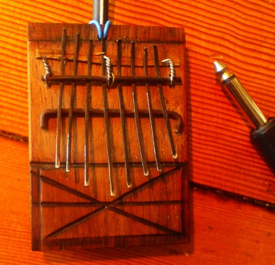
My analyser should specialise in odd sounds, like the cute
kalimba which is my favourite electro-acoustical
testing-and-doodling-toy.
|
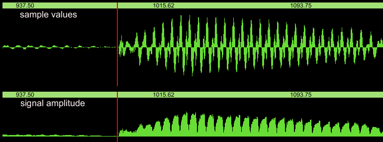
The kalimba produces very clear attacks, and at least for the eye it is easy to identify the beats:
 |
But, the computer has no eyes and it needs unambiguous instructions
about how to determine the exact location of an attack. The simplest
method would be to check for a certain sound level, since the highest
level is always at the attack. But beats are more about dynamics than
about sound level. I need to find a difference, rather than an absolute
value. The point where the sudden increase starts.
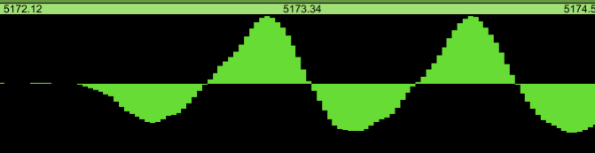
Let us look at such a point a bit closer. Here is a very clear
starting point. Yet the rise in sample values is not that sudden at
all, when viewed at this scale:
 |
Looking closer still, individual samples appear. It is from these
values that the computer must determine the beat start. But all these
cycles could look like a beat start!
 |
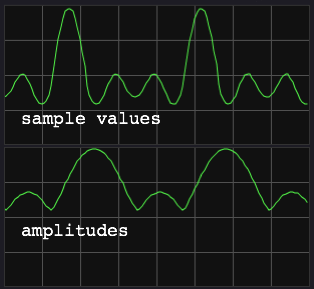
One problem is, that we see samples values and not amplitudes. These
cycles may represent a rather steady amplitude, but how do we get
amplitudes from the sample values? Amplitudes can be computed over an
interval, by taking the root of the mean of squares. This would give
some average amplitude - is that convenient? We are trying to detect a
sudden rise... There is another method, computing so called
instantaneous amplitudes. I will illustrate that method later, but let
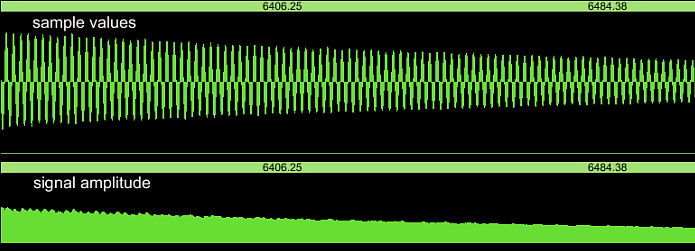
me first do an example plot of sample values versus (instantaneous)
amplitudes:
 |
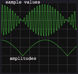
The amplitudes are not exactly constant after the attack. There is
amplitude modulation, and then I have even selected a favourable
figure. In most cases there is more modulation in the transient part.
In the decay part of the kalimba sound, the amplitude smoothly fades
away:
 |
This is a convenient phenomenon. After the dectection of an attack, a
gate for the analysis routine can be temporarily closed. A timer can be
set to open that gate after the transient part, which is relatively
short.
A practical implementation of the beat detector could thus start
with
instantaneous amplitude computation, for which a rather fascinating
method exists. The method is about the following question: if you could
create two orthogonal phases of one and the same signal, you would have
pairs of samples, and from each pair you can compute the amplitude for
that moment in time. The mathematics behind the process are
known
as Discrete Hilbert Transform. That is why you can find objects named
[hilbert~]
in Max/MSP and Pd. More details are on the page Complexify a Real Signal.
Here is a short sketch of an attack detector which uses
instantaneous amplitudes for analysis. This method is not perfect, and
it's description serves to pinpoint the major difficulty in attack
detection.
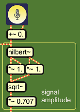 |
A signal is routed in the
Hilbert Transformer, and two orthogonal signal phases come out: a real
phase and an imaginary phase. These
are both squared, then summed, and the square root of the sum is taken:
The multiplication with 0.707 (1/sqrt(2)) is a normalisation,
because the extra phase added it's own amplitude. It was not originally
there but created as a helper signal. |
 |
The amplitudes are routed in a differentiator, because I want
to find an amplitude rise, not an amplitude value. The differentiator
output is the
amplitude difference A[n]-A[n-1]. There is also an object 'delta~'
which can do this. |
The difference of two succesive instantaneous amplitudes reflects an
amplitude slope at any sampled moment in time. It is not precisely a
tangent but that does not matter for practical purposes.
 |
 |
Next comes the thresh~ object, which sends a boolean (0. or 1.
for false or true) out, true when the input value reaches the threshold
level. There is also a hysteresis level which you can set, so the
boolean will not flip-flop rapidly around the threshold level. The
output of the thresh~ object is used as a trigger. |
Following thresh~ comes an object cuepoint~, which makes a cuepoint
from an index signal coming in it's left inlet, at the moment when a
trigger signal comes in the middle inlet. cuepoint~ will close a gate
internally after a trigger has come in. The right inlet is for a user
parameter 'refractory time' (in number of samples). This is a timer
that will open the gate again after it has counted down to zero. The
output will
send the cuepoint as a
message, not a signal.
 |
cuepoint~ is not a regular Max/MSP object, I wrote it for the
purpose. Converting a value from the signal stream to a message with
sample-precise timing is problematic, in my experience. I could not get
it fixed with whatever combination of regular objects, though I may
have overlooked possibilities. At the page bottom is a link to download
the cuepoint~ object, compiled for IntelMac. Anyway, the intention is
to store an
array of cuepoints in message form. Such an array need not be very
long. If my circular signal buffer has room for a couple dozen audio
segments, then that is also the number of cuepoints I need.
 |
Just like
the circular audio buffer is recycled by writing new samples over old
ones, the
same holds for the cuepoints: when the array is full, the oldest value
can be discarded and overwritten by the newest value. For messages,
this is what the cycle object does in Max/MSP. Here I have an array
with four cuepoints in the test patch. I can mouse-click on a cuepoint
to set a marker in the waveform at the cuepoint location, and check how
accurate the beat detection was... |
Here is one such cuepoint, as found by the beat-detection routine:
 |
Checking the same cuepoint at the scale of individual samples, it
turns out that the analyser missed only 0.2 milliseconds, ten samples.
From the figure, it is clear that the
amplitude rise is delayed respective to the sample values. That is
because the filters in the Hilbert transformer have a rise time, a kind
of mathematical inertia.
 |
Was this detection accuracy coincidental, or systematic? I checked a
lot of cuepoints from kalimba beat detection and found the results to
be systematically of equivalent accuracy. Maybe the kalimba happens to
produce the easiest targets for beat detection?
In the figure below, I pronounced the word 'beat', and what you see
is the first 150 milliseconds, the b, and the red line showing the
cuepoint:
 |
The 't' of 'beat' comes after a short silence, and it is
detected
separately:
 |
But there was also a false detection in the middle of 'bea'. That is
not surprising, there is a lot of amplitude modulation there, in
contrast with the smooth decay of a simple instrument like the kalimba.
Can I do something about that?
I tried filtering the amplitudes with a lo-pass filter to shape an
amplitude envelope. The filter smoothens the amplitude modulation, but
it
also smoothens the attack, and the detection comes way too late, if it
comes at all. Therefore, amplitude filtering is not in itself an
effective solution.
If I am to distinguish 'beat-internal' or periodic amplitude
modulation from
overall amplitude fluctuations, I better inspect it's cause and
character closely before speculating about solutions.
Here is an example showing three periods from the middle
of the word 'beat':
 |
The periodicity, both in sample values and in amplitude, is 5
milliseconds, which translates to 200 Hz. That must be the fundamental
of my regular speech, because I found that periodicity at many places
throughout the buffer.
When different frequencies sound simultaneously, amplitude
modulation will happen, caused by phase cancellation. This means that
amplitude modulation will be present in every but the simplest type of
sound material. This holds for harmonic recipes just as well as for
inharmonic sounds. Here are two examples with computer-generated
cosines to illustrate that:
 |
Here is the sum of a harmonic set of frequencies: 200, 400 and
600 Hz with equal amplitudes. The
periodicity of this wave is 200 Hz, the fundamental frequency. In harmonic recipes, the amplitude modulation will show
rectified-sinusoidal shapes. The periodicity is that of the fundamental
note, but the pattern can be quite complex. |
 |
This is an inharmonic combination of frequencies: 200 Hz and
211.89 Hz, a one note interval in equal
temperament. Theoretically, there is no fundamental period for this
particular combination because the frequencies do not share a common
integer multiple. Still, such nearly-equal frequency combinations
produce a very strong sense of periodicity, by their amplitude
modulation. The difference frequency is perceived in the modulation, in
this case (nearly) 12 Hz. With good reason, this phenomenon is called
'beat frequency'. |
Because amplitude modulation can often be perceived as a low
frequency, it is tempting to try hi-pass filtering. That does not help.
The modulations are like ghost frequencies: when you try to kill them,
it turns out they are not really there, although they keep on plaguing
you. The only way to catch them is: averaging the amplitude over a
large analysis period. The analysis should cover two (pseudo-)periods
of the lowest amplitude modulation to relieve the effect. For the
example above, with the one-note interval, that would be 6 Hz or
0.16666 seconds. A sudden amplitude rise may still be detected, even
within
such a large analysis frame, but it's exact start position can no
longer be found. That is the dilemma.
Is there a practical way to
recognise periodic amplitude modulation, and distinguish it from sudden
amplitude rise?
Of course, periodic modulation is characterised by repetition. Is such
repetition systematic enough to identify periodicity? After a lot of
experimenting, I decided to test actual amplitude against a 'peak
envelope' of
amplitudes. By the way, this may be a conventional method, even though
I have not seen it explained, so far.
 |
The peak envelope describes an exponential decay of amplitude peaks.
Everytime when an actual amplitude rises above the envelope, the
envelope is reset to that new peak value. The peak envelope of an
amplitude-modulated signal could look like this:
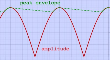 |
Periodic amplitude peaks rise above the peak envelope, but only with
a small amount. For an unambiguous attack however, the picture is
different. It looks more like this:
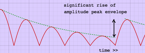 |
I found that instantaneous amplitudes are
still too variant to make
a
good peak envelope, and an amplitude average over a couple of
milliseconds
is about the minimum that works. Therefore, I said goodbye to my
beloved instantaneous amplitudes, and compute average amplitudes over
blocks of 64 samples, using the root of
mean of squares (RMS) method. The envelope decay factor is
computed from a time constant in milliseconds, like it can be done for
resonators (for more details, see
the page 'complex
resonator'):
decay_factor =
exp(-1000/samplerate/timeconstant);
It is also possible to work with deciBels,
logarithms of the energy or amplitude. That is what I did accidentally.
Below is an impression of amplitudes expressed in deciBel form.
DeciBels show a rather different curve.
 |
DeciBels are computed from energy or amplitude with:
deciBel level = 10 * log(energy / reference energy), or
deciBel level = 20 * log(amplitude / reference amplitude)
Because deciBels are logarithms of amplitudes, a ratio of amplitudes
will translate to a difference in deciBels. Or in other words, an
exponential decay of amplitudes translates to a linear decay of
deciBels. Here is an impression:
 |
Because of this translation, a peak envelope of deciBels should
theoretically be calculated by subtracting a small term, instead of
applying a decay factor. This is what I overlooked in my first
implementation with a deciBel peak envelope. Lucky me. After
discovering my mistake, I compared the wrong method with the correct
one. The wrong method turned out to perform better, in practice! It is
more sensitive to attacks, while it does not seem to produce more false
detections. Therefore, I stick to my wrong method: testing an actual
deciBel level against an exponentially decaying peak envelope of
deciBels.
Many of the amplitude modulations happen within a 64 samples frame. With
44K1 sampling rate, a 64 samples frame length represents 689 Hz.
Periodic
amplitude modulation with lower frequency is partially masked by the
peak envelope. The extent of masking is determined by the time constant
(thus decay factor).
An attack is detected when a specified difference between actual
deciBel level and peak envelope is reached or exceeded. For example:
when the
minimum difference is
defined 6 deciBel, a sound which suddenly grows twice as
loud is identified as an attack. The problem with this test is, that
low level noise can easily vary to this amount and trigger a false
detection. Therefore, the actual deciBel level must also exceed an
absolute threshold level, to pass the attack detection test.
While I am computing deciBel levels anyway, it is worthwile to test
these against a level defined as 'silence'. With this extra test, the
end of a sound segment can be identified as well, and silences can be
omitted from recording. All together, there are now three reference
levels and one reference interval:
- unity gain, the reference amplitude from which the deciBels are
computed
- absolute attack threshold in deciBels
- absolute silence threshold in deciBels
- [actual level - peak envelope level], an interval in deciBels
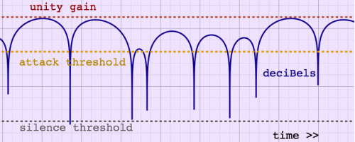 |
A definite advantage of testing against a peak envelope is the large
dynamic range covered by the analysis. Even at very low levels, attacks
can be detected, if you want. The absolute attack threshold can be used
to delimit musical attacks from unintentional clicks and pops of
instrument handling or background noises.
In practice, the deciBel peak envelope is very good at masking
periodic amplitude modulation. The plot below, of some nonsense words
spoken, shows the attack cuepoints as vertical lines. The vowels, with
their heavy amplitude modulation, do not produce false triggers with
this method.
 |
Since I work with 64-sample analysis frames now, there is an
uncertainty about the exact time position of an attack. The attack
started somewhere within a frame. That could be at the beginning of
the frame, in the middle, or at... the end? Probably not at the end,
because in that case, the attack would be detected in the next analysis
frame. So, it is even possible that the attack started just before the
frame where it was detected.
Of course, I could inspect a frame of attack detection more closely,
and try to find the attack start with better accuracy. But how? Plain
sample values tell very little about an amplitude rise. At least, the
cue must not point to an index with
substantial sample value. Therefore, I decided to keep track of
zero-crossings, and locate the cuepoint at a zero-crossing preceding
the attack detection.
Let me illustrate an example. Here is a sequence of kalimba notes,
with vertical lines indicating attack cuepoints. One of them is marked
red, and this attack interrupts a note which has not yet decayed to a
low level:
 |
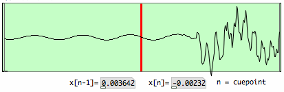
Zooming in on this spot, the position of the cuepoint is shown in a
512 point plot. The sample value of the cuepoint is printed, and the
value just before the cuepoint. Between them is a zero-crossing. It is
the ideal location for a cuepoint indeed.
 |
It is not always so ideal as in the example above. The uncertainty about the location necessitates a safety margin extending over the frame of detection and the preceding frame. Here is an example of a less ideal detection:
 |
Moreover, a low frequency component in a wave preceding the attack
can
make zero-crossings sparse, thereby enlarging the distance between a
zero-crossing and the actual attack start.
An alternative strategy would be to ignore zero-crossings, and just
apply a
short fade-in to erase the ugly blips that come with arbitrary cuts.
But, in my view, a fade-in can erase the most distinct part of
a musical sound: it's onset. In most cases, the distance from cuepoint
to actual attack is less than two blocks of 64 samples, or 3
milliseconds at 44K1 sampling rate. With a slowed down replay of the
audio fragment, the
delay increases. For example, at two octaves down, it can be up to 12
milliseconds. Although that is much more than I aimed for when starting
my
experiments, the timing error does not exceed the limits of practical
use.
Using the above described technique, a signal can be recorded into a
(circular) buffer, while attack cuepoints are stored for replay
purposes. I tried building separate loop-recorder and attack detector
object classes, for Pure Data. The result was not sample-precise, for
some
reason. Then I combined the loop-recorder and attack-detector into one
single object class, and got sample-accurate registration of cuepoints
at
zero-crossings. The data is recorded in a named buffer, so it can be
accessed for replay by other objects. For that purpose, I designed a
specialised player class, which can play a segment at any speed,
forward or backward, even if that segment wraps around the cut of the
buffer.
The record object class, titled [slicerec~], has some details which were not yet mentioned above. I found that the end of a slice, even when it ends neatly at a zero-crossing, can produce an audible blip at replay. This happens when a slice was terminated by a new attack before it decayed to a low level. While a sudden attack is a normal physical or even musical phenomenon, a sudden end is not natural.
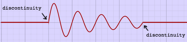 |
The sudden end is
a discountinuity, and the blip, sounding so conspicuous in the void
after the end, is undesired. Therefore I decided to apply a very short
(64 samples) fade-out to every slice, before writing these samples to
the buffer. This fade-out is implemented as the second half of a Hann
or cosine window (see the page 'FFT
window'
for details and illustrations on window functions). Despite the limited
length, this Hann type fade-out is very effective in eliminating blip
sounds.
Another point of inspection was the onset of the signal after a
period of silence. Once an attack is detected, one or two
frames of meaningful audio are already history. If periods of silence
are not recorded, the history of two frame lengths must at least be
constantly buffered, and inserted when recording is resumed. Since
recording is done framewise in the [slicerec~] object, it can not be
forced to start at a zero-crossing. A short fade-in is obligatory here.
The fade-in is 64 samples and it's shape is the first
half of a Hann window.
 |
So far, I have only described how to identify an attack in an audio
stream. For realtime applications, the sliced result should preferrably
be stored in a constantly refreshed circular buffer. Reading slices
from a circular buffer brings some peculiarities, unknown from
conventional slicers and loopers. These peculiarities are discussed on
the next page, because this text is
getting too long.
|
|
Others downloads which used to be here are replaced by a new package
Slice//Jockey.

