(page under construction)
on Hilbert Transform and all-pass filtering
Complex signals are valuable, because they offer an opportunity to
calculate instantaneous energy, amplitude and frequency. That is why
complex signals are dubbed 'analytic signals'. The signal can be
analysed sample-wise instead of frame-wise, and sometimes such fast
access to analysis is welcome.
To derive an analytic signal from a real signal, a -pi/2 radian
phase
shifted version of the real signal must be made, an imaginary phase. In
engineering terms, that extra signal is called quadrature phase,
because
pi/2 radians make a square
angle on the complex plane. The mathematics of the transform were
developed by the German
mathematician David Hilbert, hence the title Hilbert Transform.
 |
For each frequency, a -pi/2 radian phase shift translates to a known
time-shift: a quarter of a cycle in the positive direction on the
timeline, meaning [frequency/4] seconds delay. Because the time-shift
is
different for each frequency, it is not trivial to shift a compound
signal by a fixed arc length. The example below with only two harmonic
components serves to
illustrate that:
 |
It is useful to first have a look at real and complex signals in
frequency domain. Here is the spectrum of a real signal, with positive
frequencies in the lower half of the spectrum and negative frequencies
in the upper half. The spectrum is mirror-symmetric:
 |
The spectrum of a complex signal with the same frequency is
single-sided. It has only positive frequencies, filling the first half
of the spectrum up to Nyquist. Analysed with a DFT, there is always
spectral leakage and therefore the negative frequency coefficients
still have small non-zero values:
 |
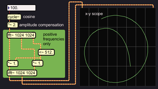
Inversely, it should be possible to get a complex signal by simply
erasing the negative frequencies from a real signal's spectrum. That is
what I am going to check with complex FFT in a Max/MSP patch. To avoid
the leakage
problem in this experiment, I tune the input test signal to an FFT
harmonic. The real and imaginary inverse FFT outputs are connected to
an
x-y scope so the orthogonality (perpendicularity) of the phases can be
checked:
 |
That works as expected. The scope trace would be elliptical or a
straight line if the phases were not orthogonal. It could be done for
arbitrary input
signals, when proper windowing and overlap is applied to the FFT.
Otherwise you get this:
 |
Below is another method to get complex phases via frequency domain.
It is done with one real FFT and two real IFFT's. The first IFFT does
the in-phase or real phase output, and the second IFFT does the
quadrature phase or imaginary phase output. The spectrum is
rotated over -pi/2 radian by feeding the FFT imaginary coefficients in
the
second IFFT real input, and the real coefficients sign-flipped in the
second IFFT imaginary input. The patch does four times overlap and Hann
windows before and after transform. The complex output is accurate for
frequencies from double the FFT fundamental up till near Nyquist.
 |
It is only for the purpose of illustration that I use an FFT to make
a real signal complex. Because in the end, I do not want to wait for
that whole FFT to happen before I have my complex signal.
To perform Hilbert Transform in time domain, must be done by
convolution. That means filtering. I need to know the filter impulse
response. A filter that makes a sine
out of each cosine by phase-shifting that cosine with -pi/2 radians.
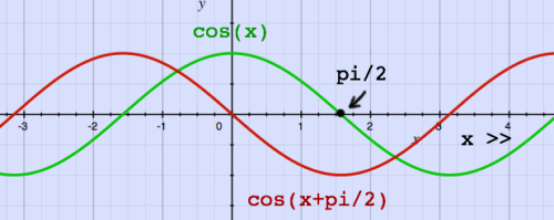
Even
this simple statement confuses me so often. Why a negative shift? Let
me
just plot this, to be shure why sin(x) = cos(x-pi/2):
 |
For Hilbert Transform, the phase shift must be done for all
frequencies, except for DC and the Nyquist frequency, which can not be
phase shifted by pi/2 rad because they are pure real. For the negative
frequencies,
cos(x) must be transformed to -sin(x). This goes:
-sin(x) = cos(x+pi/2)
 |
The phase shifts should be effectuated by convolution, but how? Again,
frequency domain can help to clarify. Convolution in time domain is
equivalent to
multiplication in frequency domain. See the pages 'Convolution' and 'Fast Convolution'
for illustrations on this topic. All -pi/2 and pi/2 phase shifts for
Hilbert Transform
could be performed in frequency domain as multiplications with -i for
positive frequencies
(in the first part of the spectrum) and i
for negative frequencies (in the second part). This is what I actually
did in the last Max/MSP patch above. -i and i are imaginary
coefficients of
magnitude -1 and 1:
 |
To find the impulse response for Hilbert Transform in time domain,
this spectrum must be inverse-FFT'd. It is first normalised, because
there would be too much energy in the impulse response otherwise. The
normalisation factor is [0.5 / N], where 0.5 accounts for the fact that
the correlation weight is distributed over positive and negative
frequencies. After IFFT, this pure real signal is
the result:
 |
The impulse response for a Hilbert Transform filter is 1/pi*x, but
only for uneven x. It represents a sum of sinewaves. The impulse
response is not by nature restricted to a defined
length.
Even when the time frame will be confined to a practical length of
choice, the
left side of the impulse response poses a problem. That part of the
filter is non-causal, it has points in negative time, meaning that we
have to collect a corresponding number of samples in a delay line
before they can be processed. Implementing this as a Finite Impulse
Response filter, would just be the slow convolution version of the
spectrum manipulation showed earlier. Of course, this would not bring
any advantage.
Probably I should be prepared for another compromise. If I can live
with a real and imaginary phase which are both phase-shifted respective to
the input signal, the complexification can be done with help of
phase-shifting all-pass filters. This is not Hilbert Transform in the
proper sense,
since it does not produce a phase orthogonal to the input. Anyhow, if
the output phases show a 90 degree phase difference, it will
do fine for my analysis purposes.
This is actually a completely different route to get complex
signals, so I will start from scratch. Digital time domain filters add
delayed input- and/or output values to the signal, eventually with a
scaling factor and/or sign-flip inbetween. The phase-shift effect of
delaying a stream of sample values varies per frequency. DC can not be
phase-shifted by delay. With a one sample delay, positive frequencies
are shifted by an angle inbetween zero and -pi radians:
 phase shifts of frequencies when one sample delayed |
A sign-flip does a rotation over pi radian for all frequencies. The
combination of one sample delay and sign-flip has this spectral effect:
 phase shifts of frequencies one sample delayed and sign-flipped |
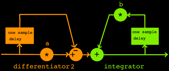
One sample delay and sign-flip is applied in differentiators. And
differentiators, combined with integrators, can make all-pass filters
under certain conditions. A
differentiator is a feed-forward filter. It looks a bit like the
integrator figuring on the previous pages, but there is no
recirculation, and the delayed/scaled
sample is subtracted from the input, instead of summed to it. Here is a
differentiator/integrator flow graph:
 y[n] = x[n] - a*x[n-1] + b*y[n-1] |
Since integration is the inverse process of
differentiation, the filtering effect of the differentiator could be
undone by the integrator when their coefficients a and b were set to
the same
value. For all frequencies, DC included, the amplitude and phase
response of
the filter combination would be flat at unity amplitude and phase zero.
Of
course, such a filter without any effect would be of no use, and in
practical applications the coefficients would have different values to
render desired filter effects. I just mentioned the do-nothing filter
as a comparison for what comes next: the alternative differentiator
type.
It's filter coefficient is not in the feed-forward line, but directly
on the input:
 |
Implemented this way, the differentiator has the same amplitude
response as the earlier sketched one, but the phase response is
altered. So we have two differentiator types. When x[n] is the
differentiator input and y[n] is it's output, the following filter
expressions apply to them:
y[n] = x[n] - a*x[n-1] differentiator type 1
y[n] = a*x[n] - x[n-1] differentiator type 2
I will plot example phase spectra for the two types to illustrate
the spectacular difference between them. For the moment, the integrator
is not taken into consideration. I use Max/MSP's filtergraph~ object to
compute and plot the spectra. The filter coefficient 'a' is 0.9 in both
cases. Here is the phase response of differentiator type 1:
 differentiator type 1 with: y[n] = x[n] - 0.9*x[n-1] |
And here is the response of differentiator type 2:
 differentiator type 2 with: y[n] = 0.9*x[n] - x[n-1] |
To demonstrate what the differentiator types do in combination with
an integrator, I first plot the integrator phase response separately.
Here it is, for filter coefficient b=0.9:
 integrator with: y[n] = x[n] + 0.9*y[n-1] |
The curve is exactly the inverse of the differentiator type 1 curve.
These
phase shifts will cancel each other in a combined filter. I am not
going to plot the flat phase response resulting from that, a dull line
at phase zero.
In contrast, the differentiator-type2/integrator combination add
their phase-shifts. Instead of a
do-nothing filter, you have a
leave-the-amplitudes-but-shift-the-phases filter, concisely called
all-pass filter. The net phase response with coefficient 0.9 looks like
this:
 all-pass filter with: y[n] = 0.9*x[n] - x[n-1] + 0.9*y[n-1] |
The same all-pass trick can be done with two samples delay time (or
more, like is done in reverb simulation). The filter flow graph remains
the same, only the delay time is increased:
 y[n] = a*x[n] - x[n-2] + b*y[n-2] |
Using two samples delay instead of one sample, is equivalent to downsampling the filter's time resolution with a factor 2. The total phase shift over the spectrum is doubled, as compared to the all-pass filter with one sample delay:
 all-pass filter with: y[n] = 0.9*x[n] - x[n-2] + 0.9*y[n-2] |
There is also the option to use one and two samples delay combined
in an all-pass biquad filter, which has this signal flow graph:
 |
Each section has two delays and three coefficients. The b0
coefficient is often factored out for efficiency reasons.
It
is not so obvious how the coefficients should be set equal for both
sections, to make an all-pass filter. This
deserves special attention. The a and b coefficients should be treated
as vectors, arrays. The b vector must be computed first, and then
time-reversed to find the a
vector. The b coefficients translate to the a
coefficients in the following way:
 |
A two-pole two-zero all-pass filter is thus characterized by these
equalities:
a0 = b2
a1 = b1
a2 = b0
Below is an example of what the biquad all-pass can do to the phase
spectrum. The phase-wrap that was at DC with the simpler filter is now
duplicated. It indicates the filter center frequency, since half of the
phase-shift is between DC and the phase-wrap, while the other half is
between the wrap and Nyquist. With a biquad all-pass, the center
frequency can be positioned at any location of choice within the
spectrum.
 all-pass filter: y[n] = 0.2*[x] - 0.9*x[n-1] + x[n-2] + 0.9*y[n-1] - 0.2*y[n-2] |
Whatever all-pass
filter type and coefficients we use, the shift at DC
and Nyquist frequency will always be zero, pi radian, or a multiple of
pi. The phase response is tied like cymbalom strings to the pi radian
grid.
Flexible
strings they are, but a pure -pi/2 radian phase shift for all
frequencies is certainly out of the question.
The only thing we can do is to deform two 'strings', phase responses, in such a way that they are approximately parallel over a maximized portion of their length.
 |
To accomplish this, one all-pass filter per output phase is not
enough. For each phase, there must be a cascade of them. In itself, a
cascade is not a complicated concept. It just means that there are two
ore more filters in series, like here:
 |
The
phase shift of the cascade is just the sum of all the filter's shifts.
Nonetheless, the math involved in cascade coefficient
calculation is complicated, and generally left to specialised filter
design software. For a start, I will review a couple of methods which
were published with coefficients included, and compare these.
With only two biquads in cascade per phase, it is already possible
to complexify real signals over a wide range of frequencies. Pure Data
has this method as a patch, so we can see how it is implemented and
learn from it. In the pd patch below, the cascades are positioned in
such a way that they give
positive frequencies. A modulated square wave serves as test input
signal. The full complex spectrum shows that the negative
frequencies are gone indeed:
 |
The output of this constellation is approximately orthogonal
starting from around 80 Hz (at sampling rate 44K1) till half the
Nyquist frequency. After Nyquist/2 there is a gradual decrease in the
phase interval, and near Nyquist the outputs show zero phase
difference. Max/Msp's hilbert~ object may have a procedure comparable
to pd's hilbert~. It's accuracy in the low spectrum half is better.
Possibly it has more filters per cascade, but the object source is not
public so it can not be compared. When implemented in C, each all-pass
biquad can be efficiently computed as:
y[n] = a0*(x[n]+y[n-2])
+ a1*(y[n-1]-x[n-1]) +
x[n-2]
With two multiplications per biquad, and a minimum of 2x2 biquads, a
complex signal can be computed at a minimum price of 8
multiplications plus a number of additions / subtractions.
It seems that the elementary two-sample delay all-pass filters,
sketched earlier on this page, are
popular building blocks in the multirate filtering scene. Let me redraw
the differentiator / integrator combination as an all-pass yin and yang
unit to illustrate it's elegance and efficiency:
 y[n] = a*(x[n] + y[n-2]) - x[n-2] |
Cascades of them are used in arrays, where each cascade represents a separate phase. Theoretically there can be any number of cascades, and therefore any number of phases. That is why the concept is called 'Polyphase Infinite Impulse Response', abbreviated polyphase IIR. A dual-phase version of the polyphase IIR principle, with it's possible output signals, can be sketched like this:
 |
The combined output of different all-pass filter cascades can produce an amplitude filtering effect as result of phase cancellations and summations. At first sight, this seems an elaborate way to implement a filter. But it is actually efficient because of the one-coefficient units inside. The polyphase set-up offers interesting options, like extracting sum and difference output with complementary spectra, and phase decomposition before the filters. A typical application is halfband filtering for a downsampling filterbank. If you want to search the internet on this topic, do not forget the IIR term, because there is also polyphase FIR, and both are used in multirate filtering. Many texts on polyphase IIR are by Artur Krukowski and Izzet Kale.
The technique can also be applied to produce output phases with pi/2
phase interval. That is why I mention it here, of course. Coefficients
for 4-section cascades are calculated and published by
Olli Niemitalo on http://yehar.com/blog/.
It was also his presentation that put me on the track of polyphase IIR.
I tried Olli's filters in Max/MSP, using biquads. The
one-sample delay coefficients are just set to zero. I swapped Olli's
first and second cascades to get positive frequencies. Here is the Max
patch with a
modulated square wave as input and showing the full spectrum of the
complex output:
 Max/Msp's biquad~ has: y[n] = a0*x[n]+a1*x[n-1]+a2*x[n-2]-b1*x[n-1]-b2*x[n-2] |
Notice that this routine could be done with a total of 8
multiplications as well. Compared to Pure Data's
implementation, Olli's filters produce a better complex signal. Phase
orthogonality starts around 40 Hz (at 44K1 sampling rate). The
specifications show symmetry over Nyquist/2, therefore this transform
is also quite accurate in the highest frequency range. The figure below
shows a comparison at 18000 Hz. The lines in the scope traces are just
interpolations between the actual datapoints.
 |
Although regular audio has little energy in the highest frequency
range, this can be different for
certain (manipulated) signals.
All toghether, polyphase IIR seems more
promising to me than the classic biquad method. That is why I want to
find more details of this technique. How to design a polyphase IIR
Hilbert Transformer of higher order? Laurent de Soras has published a
C++ resampling library using polyphase IIR halfband filtering, with
pi/2 phaser functions as a bonus. See http://ldesoras.free.fr/index.html.
I am now examining this library too see if and how it can be applied
for analysis in a real time system like Max/MSP or Pure Data. This page
will be updated as soon as I have results.