(download Pure Data patches at page bottom)
In my live performance tool Instant Decomposer I use amplitude
compression and limiting at several points in the signal flow. At the
input side, it helps my voice to sound closer and more detailed. At
other points it regulates submix levels. While I am doing amplitude
regulation anyway, I take the opportunity to expand the lowest
amplitude range and thereby attenuate background noise. The compander
is an expander/compressor/limiter. This is all done with an
experimental technique using an analytic signal, to which the title
'quadrature compander' refers.
Below is an example plot of input-output amplitude mapping with
expansion, compression and limiting in one smooth curve, as compared to
linear amplification.
|
At this point, it is important to define 'signal amplitude', the
entity to be mapped from input to output with a non-linear curve. The
regular way of computing amplitude of an arbitrary signal is by
computing
the root of mean of squared sample values (RMS) over a specified time
interval. That time interval should match the lowest audio-frequencies
in the signal, to avoid falsely recorded amplitude modulation.
There is also a method to compute instantaneous
amplitudes, with help of an analytic signal. An analytic signal
consists of two phases, the second of which is sometimes called
quadrature phase. Hence the title quadrature compander. Apart from the
popular frequency shifter, this was the first occasion
where an analytic signal appeared to be of practical use for me. The
advantage of instantaneous amplitudes is the fast detection of a
sudden amplitude rise.
Methods
to derive analytic signals are discussed on the page 'complexify
a real signal'. For the quadrature compander (and anywhere else) I
use the IIR all-pass filter method. Below is an example plot of
amplitude computation done with the IIR method. The amplitude curve
shows an overshoot effect at the attack, caused by the recursive
filters:
 amplitude with analytic signal |
For comparison, here is the same signal, and it's amplitude now
measured with the RMS method:
 amplitude with RMS method |
The RMS method cannot be precise in time, because it works with
signal blocks. But with the analytic signal method, there is a delay in
the measurement as well. That delay is frequency-dependant, caused by
the IIR filter response. The amplitude peak seems to be delayed by half
a cycle when I take a closer look:
 amplitude with analytic signal |
Since the measurement delay with the analytic signal is
frequency-dependant, there is no practical way to sync the amplitude
curve with the original signal. To cut things short, I decided to use
the analytic signal itself as the audio, by summing real and imaginary
phases and reduce the resultant amplitude with factor 1/sqrt(2). Then,
the measured amplitude will by definition always exactly match the
processed signal.
This procedure will completely ruin the phase relations within the
signal. A cardinal sin in dsp land. Will the summation of the real and
imaginary phase not cause phase cancellations, and thereby reduce or
even eliminate some frequencies? No, it will not, because real and
imaginary phases are orthogonal, and thus complementary in the
summation. Further down, I will discuss the implications in more
detail. For the moment, I will just employ my brutal shortcut and
continue with the amplitude compander.
All compound signals, harmonic recipes included, display amplitude
modulation. The amplitude compander must be made insensitive to
periodic amplitude modulation. With the RMS method, this can be done
simply by selecting the appropriate time interval: twice the period of
the lowest harmonic tones in the signal. That can be quite long.
When using instantaneous amplitudes, periodic amplitude modulations
are a real pain. They must somehow be ignored by the amplitude
calculator. Both the problem and a solution are illustrated on the page
'Slicing Odd Beats',
where I was doing attack detection. The trick is to use a peak envelope
of the amplitude. The peak envelope of periodic amplitude modulation
looks like this:
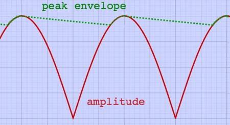 |
With the amplitude peak envelope, a sudden amplitude rise will be
followed with precision, while periodic modulation will be smoothed to
an extent of choice. The time constant in the enveloper sets the
envelope decay ratio, and thus the smoothing effect. The amplitude
envelope of even the freakiest signals can be approximated this way:
 |
Next thing is the design of input-output amplitude mapping curves. As
the example plot on top of page showed, noise suppression, signal
compression and limiting can be done in one smooth curve. I want that
curve to be calculated from a couple of parameters:
1. compander factor
2. rotation point
For ease of use, the signal is always limited to y = 1. Compander
factor is the output gain factor at the limiter start point. Rotation
point is the lower point where x = y, separating the attenuation range
from the amplification range. Here is the earlier example plot once
more, showing a compander factor 1 and rotation point at amplitude 0.18:
|
With these two parameters, it is very easy to set the curve in such a
way that microphone noise is below the rotation point, and thus
attenuated. However, the amount
of attenuation is dependant on the compander factor, and so is the
amount of amplification above the rotation point. Here is a more
extreme setting with compander factor 2 and rotation point at amplitude
0.1:
 |
Here is how these curves are computed. All y values for x above the
limiter start point are just set to 1. The limiter start point is at x
= 1 / compander factor. In the plot above it is at x = 0.5. The smooth
curve proper is a quarter of a sine cycle (with angle 0.5 * pi *
compander factor, in radians) raised to a power. The exponent is a
function of both rotation point and compander factor. All taken
together:
y = sin(companderfactor*0.5*pi*x)^exponent for x <=
1/companderfactor
y = 1 for x > 1/companderfactor
exponent =
log(rotationpoint)/log(sin(companderfactor*rotationpoint*0.5*pi))
One disadvantage of fast compression/limiting can be the muffling of
transients. Compressed percussion may sound less powerful. Therefore it
is sometimes opportune to deliberately slow down the compander response
a bit, and let transients pass with their full strength. For similar
reason, compressor release time can be slowed down. Transient peaks are
then followed by an amplitude depression, making the peaks stand out.
Such producer tricks make sounds interact with each other, and even a
limited set of sounds can result in lively music.
My quadrature compander has no separate attack and release settings.
But I can slow down response time by using a lo-pass filter on the
amplitude peak envelope. The result is a clearly defined attack in
percussive sounds. In the example below, I have clipped the attack to
create a punch effect:
 punch in the output |
The recovery time of the quadrature compander can be extended by
setting a high value for the peak envelope time constant. Combined with
high compander factor, this setting will result in a 'suck' effect like
plotted here:
 |
With only four user parameters the quadrature compander is complete. I
have implemented the scheme as a Pure Data abstraction [qompander~].
It's use is straightforward. The rotation point parameter is called
compander point and for ease of use it is set in deciBel with a range
of -96 till -20 dB.
 |
Here is the inside of the [qompander~] abstraction:
 [qompander~] abstraction |
The patch contains some subroutines, of which [pd exponent] and [pd
mapping] are shown below. The subroutine [pd pyth] does pythagoras to
find the amplitude.
 subroutine [pd exponent] |
 subroutine [pd mapping] |
[pd olli~] is my Pd implementation of Olli
Niemitalo's quadrature
transformer, using biquads. This could be done much more efficient in a
specialised Pd class but I have not done that yet.
 subroutine [pd olli~] |
You can download [qompander~] and a help patch from the page bottom
and use it if you have Pure Data installed.
Higher up I mentioned my brutal shortcut which came in handy for the
quadrature compander: summing the phases of an analytic signal and
using this as the audio. Phase relations within the signal will be
heavily distorted by this action, which is reflected in an altered
waveform. It is funny that I have never heard a difference though.
Let's see what is going on.
Below is an example of a signal with two harmonic frequency
components which I ran through the quadrature summator.
 280 + 560 Hz signal with phase rotations |
Input and output sound completely identical, although their
waveshapes differ. The frequency content has not changed. I know that
the ears and brains are not sensitive to static phase information, but
then why are dsp engineers always so zealous when it comes to linear
phase filtering? Well, it is clear that you cannot recombine the output
with the original. There will be phase cancellation effects, and thus
unintended filtering. That is one thing. You must not use the original
signal and the quadrature compander output in parallel.
Further I noticed that the onset of a sound has a different
character, at least visually. Here is again a sinewave resonator
starting neatly from 0 radians, and it's phase rotated version:
 60 Hz sinewave resonator with phase rotation |
When I compare these sounds in ideal listening conditions, I notice
a subtile increase in high frequency content at the attack, caused by
the tiny blob that arose from the phase rotation. This effect is so
minute, that I can not perceive it in normal music listening
situations. But when the signal is heavily compressed, such artefacts
become noticeable.
If
you want to do 'parallel compression' with the quadrature compander, an
extra action is required. Just like you would normally account for the
latency of a compressor, by adding equivalent delay to the original
signal, you would now add the analytic summator routine to the original
signal. Or else you could run the original signal through a second
quadrature compander with moderate settings.
I am quite satisfied with the quadrature compander, particularly
because of it's fast response. Therefore I will put up with the
inconvenience of phase rotations and use an extra compander in case of
parallel processing.
Download Pure Data patches here:
|
|
|
|
